LDA V.S. Logistic Regression:
- When the classes are well-separated, the parameter estimates for the logistic regression model are surprisingly unstable. Linear discriminant analysis does not suffer from this problem.
- If n is small and the distribution of the predictors X is approximately normal in each of the classes, the linear discriminant model is again more stable than the logistic regression model.
- Linear discriminant analysis is popular when we have more than two response classes.
Using Bayes’ Theorem for Classification
Suppose that we wish to classify an observation into one of K classes, where K ≥ 2.
Prior:Let $\pi_k=Pr(Y=k)$ represent the overall or prior probability that a randomly chosen observation comes from the kth class. This is the probability that a given observation is associated with the kth category of the response variable Y .
Let $f_k(X) ≡ Pr(X = x|Y = k)$ denote the density function of X for an observation that comes from the kth class. In other words, fk(x) is relatively large if there is a high probability that an observation in the kth class has X ≈ x.
Bayes’ theorem states that $$ \begin{align} Pr(Y=k|X=x)=\frac{\pi_k f_k(x)}{\sum_{l=1}^K\pi_lf_l(x)} \end{align} $$ Posterior:$p_k(X) = Pr(Y = k|X)$ an observation X = x belongs to the kth class, given the predictor value for that observation
Estimating $π_k$: simply compute the fraction of the training observations that belong to the kth class.
Estimating $f_k(X)$: more challenging
Linear Discriminant Analysis for p = 1
Assume p = 1—that is, we have only one predictor. We would like to obtain an estimate for $f_k(x)$ that we can estimate $p_k(x)$. We will then classify an observation to the class for which $p_k(x)$ is greatest.
Assumptions
In order to estimate $f_k(x)$, we will first make some assumptions about its form:
- Assume that $f_k(x)$ is normal or Gaussian. $$ \begin{align} f_k(x)=\frac{1}{\sqrt{2\pi}\sigma_k}\exp{\left( -\frac{1}{2\sigma_k^2}(x-\mu_k)^2 \right)} \end{align} $$
where $μ_k$ and $σ_k^2$ are the mean and variance parameters for the kth class.
- Assume that $\sigma_1^2=…=\sigma_k^2$ : that is, there is a shared variance term across all K classes, which for simplicity we can denote by $\sigma^2$.
So $$ \begin{align} p_k(x)=\frac{\pi_k \frac{1}{\sqrt{2\pi}\sigma}\exp{\left( -\frac{1}{2\sigma^2}(x-\mu_k)^2 \right)}}{\sum_{l=1}^K\pi_l\frac{1}{\sqrt{2\pi}\sigma}\exp{\left( -\frac{1}{2\sigma^2}(x-\mu_l)^2 \right)}} \end{align} $$ The Bayes classifier involves assigning an observation X = x to the class for which $p_k(x)$ is largest. Taking the log of $p_k(x)$ and rearranging the terms, it is not hard to show that this is equivalent to assigning the observation to the class for which $$ \begin{align} \delta_k(x)=x\frac{\mu_k}{\sigma^2}-\frac{\mu_k^2}{2\sigma^2}+\log(\pi_k) \quad\quad (4.13) \end{align} $$ is largest.
For instance, if K = 2 and π1 = π2, then the Bayes classifier assigns an observation to class 1 if $2x (μ_1 − μ_2) > μ^2_1 − μ^2_2$, and to class 2 otherwise. In this case, the Bayes decision boundary corresponds to the point where $$ \begin{align} x=\frac{\mu_1^2-\mu_2^2}{2(\mu_1-\mu_2)}=\frac{\mu_1+\mu_2}{2} \end{align} $$
Parameters Estimation
In practice, even if we are quite certain of our assumption that X is drawn from a Gaussian distribution within each class, we still have to estimate the parameters $μ_1, . . . , μ_K, π_1, . . . , π_K$, and $σ^2$.
Linear discriminant analysis (LDA) method approximates the Bayes classifier by plugging estimates for $μ_1, . . . , μ_K, π_1, . . . , π_K$, and $σ^2$ into (4.13)
$$ \begin{align} \hat{\mu}k=\frac{1}{n_k}\sum{i:y_i=k}x_i \quad (4.15) \ \hat{\sigma}^2=\frac{1}{n-K}\sum_{k=1}^K\sum_{i:y_i=k}(x_i-\hat{\mu_k})^2 \quad (4.16)\ \hat{\pi_k}=\frac{n_k}{n} \end{align} $$
where n is the total number of training observations, and $n_k$ is the number of training observations in the kth class.
$\hat{\mu}_k$: average of all the training observations from the kth class;
$\hat{\sigma}^2$: a weighted average of the sample variances for each of the K classes.
$\hat{\pi_k}$: the proportion of the training observations that belong to the kth class
LDA classifier
The LDA classifier assigns an observation X = x to the class for which
$$ \begin{align} \hat{\delta}_k(x)=x\frac{\hat{\mu}_k}{\hat{\sigma}^2}-\frac{\hat{\mu}_k^2}{2\hat{\sigma}^2}+\log(\hat{\pi}_k) \end{align} $$ is largest.
The word linear in the classifier’s name stems from the fact that the discriminant functions $\hat{\delta}_k(x)$ are linear functions of x.
The right-hand panel of Figure 4.4 displays a histogram of a random sample of 20 observations from each class.
To implement LDA,
- Estimating πk, μk, and σ2 using (4.15) and (4.16).
- Compute the decision boundary, shown as a black solid line, that results from assigning an observation to the class for which $\hat{\delta}_k(x)$ is largest.
In this case, since n1 = n2 = 20, we have $\hat{\pi_1}$ = $\hat{\pi_2}$. As a result, the decision boundary corresponds to the midpoint between the sample means for the two classes,$\frac{\mu_1+\mu_2}{2}$
Linear Discriminant Analysis for p >1
Assume that X = (X1,X2, . . .,Xp) is drawn from a multivariate Gaussian (or multivariate normal) distribution, with a class-specific mean vector and a common covariance matrix.
Multivariate Gaussian Distribution
Assumes that each individual predictor follows a one-dimensional normal distribution with some correlation between each pair of predictors.
To indicate that a p-dimensional random variable X has a multivariate Gaussian distribution, we write X ∼ N(μ,Σ). Here E(X) = μ is the mean of X (a vector with p components), and Cov(X) = Σ is the p × p covariance matrix of X. Formally, the multivariate Gaussian density is defined as $$ \begin{align} f(x)=\frac{1}{\sqrt{(2\pi)^{p}|Σ|}}\exp{\left( \frac{1}{2}(x-\mu)^TΣ^{-1}(x-\mu) \right)} \end{align} $$ In the case of p > 1 predictors, the LDA classifier assumes that the observations in the kth class are drawn from a multivariate Gaussian distribution $N(μ_k,Σ)$, where $μ_k$ is a class-specific mean vector, and Σ is a covariance matrix that is common to all K classes.
Plugging the density function for the kth class, $f_k(X = x)$, into $Pr(Y = k|X = x)$, the Bayes classifier assigns an observation X = x to the class for which $$ \begin{align} \delta_k(x)=x^TΣ^{-1}\mu_k-\frac{1}{2}\mu_k^TΣ^{-1}\mu_k+\log{\pi_k} \quad \quad (4.19) \end{align} $$ is largest.
Once again, we need to estimate the unknown parameters $μ_1, . . . , μ_K$, $π_1, . . . , π_K$, and Σ; the formulas are similar to those used in the one dimensional case, given in (4.15). To assign a new observation X = x, LDA plugs these estimates into (4.19) and classifies to the class for which $\hat{\delta}_k(x)$ is largest.
Overall, the LDA decision boundaries are pretty close to the Bayes decision boundaries, shown again as dashed lines.
Caveats
Training error rates will usually be lower than test error rates. The higher the ratio of parameters p to number of samples n, the more we expect this overfitting to play a role.
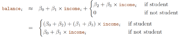
Second, since only 3.33% of the individuals in the training sample defaulted, a simple but useless classifier that always predicts that each individual will not default, regardless of his or her credit card balance and student status, will result in an error rate of 3.33%. In other words, the trivial null classifier will achieve an error rate that is only a bit higher than the LDA training set error rate.
Two Types of Error, Confusion Matrix
Binary classifier can make two types of errors:
- it can incorrectly assign an individual who defaults to the no default category;
- it can incorrectly assign an individual who does not default to the default category.
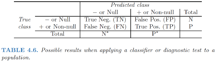
Confusion Matrix
*注意这张图不是标准的confusion matrix,看下面那张
Explanation: The matrix table reveals that LDA predicted that a total of 104 people would default. Of these people, 81 actually defaulted and 23 did not.
Type I Error: Of the 333 individuals who defaulted, 252 (or 75.7%) were missed by LDA. So while the overall error rate is low, the error rate among individuals who defaulted is very high. From the perspective of a credit card company that is trying to identify high-risk individuals, an error rate of 252/333 = 75.7% among individuals who default may well be unacceptable.
Type II Error:Only 23 out of 9, 667 of the individuals who did not default were incorrectly labeled. This looks like a pretty low error rate!
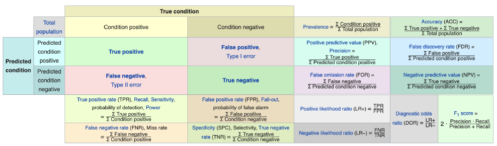
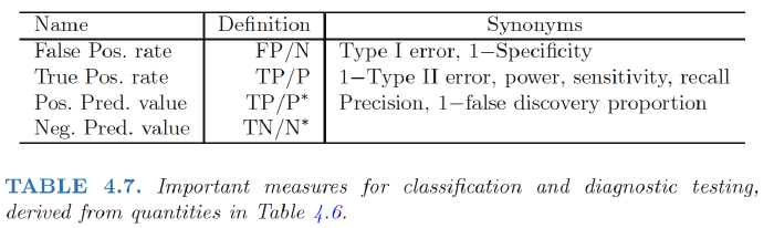
Sensitivity:the percentage of true defaulters that are identified, a low 24.3% in this case.
Specificity:the percentage of non-defaulters that are correctly identified, here (1 − 23/9, 667)× 100 = 99.8%.
Why does LDA do such a poor job of classifying the customers who default?
In other words, why does it have such a low sensitivity?
LDA is trying to approximate the Bayes classifier, which has the lowest total error rate out of all classifiers (if the Gaussian model is correct). That is, the Bayes classifier will yield the smallest possible total number of misclassified observations, irrespective of which class the errors come from.
The Bayes classifier works by assigning an observation to the class for which the posterior probability pk(X) is greatest. In the two-class case, this amounts to assigning an observation to the default class if $Pr(default = Yes|X = x) > 0.5.$
Thus, the Bayes classifier, and by extension LDA, uses a threshold of 50% for the posterior probability of default in order to assign an observation to the default class.
Modify LDA
If we are concerned about incorrectly predicting the default status for individuals who default, then we can consider lowering this threshold.
$$P(default = Yes|X = x) > 0.2$$
Figure 4.7 illustrates the trade-off that results from modifying the threshold value for the posterior probability of default
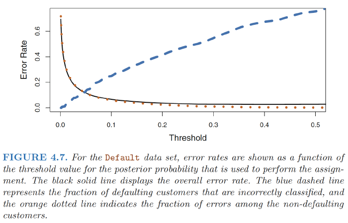
How can we decide which threshold value is best? Such a decision must be based on domain knowledge, such as detailed information about the costs associated with default.
ROC & AUC
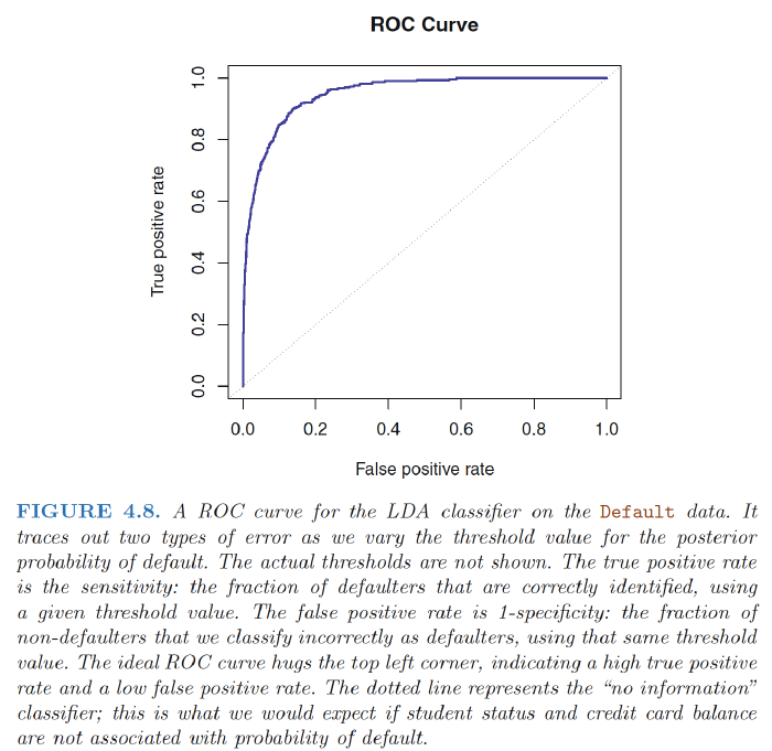
ROC:The ROC curve is a popular graphic for simultaneously displaying the two types of errors for all possible thresholds.
AUC: The overall performance of a classifier, summarized over all possible thresholds, is given by the area under the (ROC) curve (AUC).
An ideal ROC curve will hug the top left corner, so the larger the AUC the better the classifier. We expect a classifier that performs no better than chance to have an AUC of 0.5
ROC curves are useful for comparing different classifiers, since they take into account all possible thresholds.
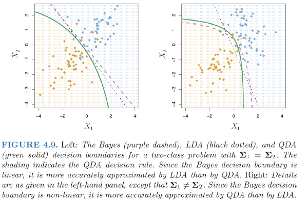
Quadratic Discriminant Analysis
Quadratic discriminant analysis (QDA) classifier results from assuming that the observations from each class are drawn from a Gaussian distribution, and plugging estimates for the parameters into Bayes’ theorem in order to perform prediction.
However, unlike LDA, QDA assumes that each class has its own covariance matrix. That is, it assumes that an observation from the kth class is of the form $X ∼ N(μ_k,Σ_k)$, where $Σ_k$ is a covariance matrix for the kth class. Under this assumption, the Bayes classifier assigns an observation $X = x$ to the class for which
$$ \begin{align} \delta_k(x)&=-\frac{1}{2}(x-\mu_k)^TΣ_k^{-1}(x-\mu_k)-\frac{1}{2}\log{|Σ_k|}+\log{\pi_k} \\ &=-\frac{1}{2}x^TΣ_k^{-1}x+x^TΣ_k^{-1}\mu_k-\frac{1}{2}\mu_k^TΣ_k^{-1}\mu_k-\frac{1}{2}\log{|Σ_k|}+\log{\pi_k} \end{align} $$
is largest.
So the QDA classifier involves plugging estimates for $Σ_k, μ_k, π_k$ into $\delta_k(x)$, and then assigning an observation $X = x$ to the class for which this quantity is largest. Unlike LDA, the quantity $x$ appears as a quadratic function.
Why does it matter whether or not we assume that the K classes share a common covariance matrix?
The answer lies in the bias-variance trade-off:
- When there are p predictors, then estimating a covariance matrix requires estimating p(p+1)/2 parameters. QDA estimates a separate covariance matrix for each class, for a total of Kp(p+1)/2 parameters.
- Consequently, LDA is a much less flexible classifier than QDA, and so has substantially lower variance.
- But there is a trade-off: if LDA’s assumption that the K classes share a common covariance matrix is badly off, then LDA can suffer from high bias.
Conclusion
- LDA tends to be a better bet than QDA if there are relatively few training observations and so reducing variance is crucial.
- QDA is recommended if the training set is very large, so that the variance of the classifier is not a major concern, or if the assumption of a common covariance matrix for the K classes is clearly untenable

Ref:
James, Gareth, et al. An introduction to statistical learning. Vol. 112. New York: springer, 2013.
Hastie, Trevor, et al. “The elements of statistical learning: data mining, inference and prediction.” The Mathematical Intelligencer 27.2 (2005): 83-85