Dimension Reduction Methods
Subset selection and shrinkage methods all use the original predictors, X1,X2, . . . , Xp.
Dimension Reduction Methods transform the predictors and then fit a least squares model using the transformed variables.
Approach
Let $Z_1,Z_2, . . . ,Z_M$ represent $M < p$ linear combinations of our original $p$ predictors. That is,
$$ \begin{align} Z_m=\sum_{j=1}^p\phi_{jm}X_j \end{align} $$
for some constants $φ_{1m}, φ_{2m} . . . , φ_{pm}, m = 1, . . .,M.$ We can then fit the linear regression model $$ \begin{align} y_i=\theta_0+\sum_{m=1}^M\theta_m z_{im}+\epsilon_i \quad i=1,2,3,4,…,n \end{align} $$ Dimension reduction: reduces the problem of estimating the $p+1$ coefficients $β_0, β_1, . . . , β_p$ to the simpler problem of estimating the $M + 1$ coefficients $θ_0, θ_1, . . . , θ_M$, where M < p. In other words, the dimension of the problem has been reduced from $p + 1$ to $M + 1$. $$ \begin{align} \sum_{m=1}^M\theta_m z_{im}&=\sum_{m=1}^M\theta_m \sum_{j=1}^p\phi_{jm}x_{ij}=\sum_{m=1}^M\sum_{j=1}^p\theta_m \phi_{jm}x_{ij}=\sum_{j=1}^p \beta_jx_{ij} \ \beta_j&=\sum_{m=1}^M\theta_m \phi_{jm} \end{align} $$ All dimension reduction methods work in two steps:
- The transformed predictors $Z_1,Z_2, . . . ,Z_M$are obtained.
- The model is fit using these $M$ predictors. However, the choice of $Z_1,Z_2, . . . ,Z_M$, or equivalently, the selection of the $φ_{jm}$’s, can be achieved in different ways.
Principal Components Regression
An Overview of Principal Components Analysis
Principal component analysis (PCA) refers to the process by which principal components are computed, and the subsequent use of these components in understanding the data.
- PCA also serves as a tool for data visualization (visualization of the observations or visualization of the variables).
What Are Principal Components?
PCA :finds a low-dimensional representation of a data set that contains as much as possible of the variation
Each of the dimensions found by PCA is a linear combination of the $p$ features.
The first principal component of a set of features $X_1,X_2, . . . , X_p$ is the normalized linear combination of the features $$ \begin{align} Z_1=\phi_{11}X_1+\phi_{21}X_2+,,,+\phi_{p1}X_p \end{align} $$ that has the largest variance.
Normalized: $\sum_{j=1}^p \phi_{j1}^2=1$
Loadings: $\phi_{11}, . . . , \phi_{p1}$ the loadings of the first principal component;
- Together, the loadings make up the principal component loading vector, $\phi_1=(\phi_{11},\phi_{21},…,\phi_{p1})^T$
1st Principal Component
Interpretation 1: greatest variability
The first principal component direction of the data: is that along which the observations vary the most.
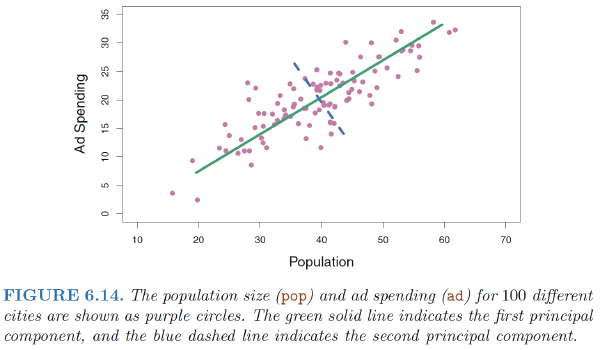
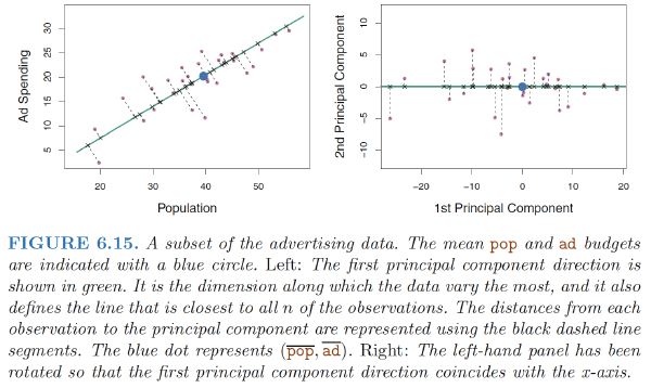
The first principal component direction is the direction along which there is the greatest variability in the data. That is, if we projected the 100 observations onto this line (as shown in the left-hand panel of Figure 6.15), then the resulting projected observations would have the largest possible variance
The first principal component is given by the formula
$$ \begin{align} Z_1 = 0.839 × (pop − \bar{pop}) + 0.544 × (ad − \bar{ad}) \end{align} $$ Here $φ_{11} = 0.839$ and $φ_{21} = 0.544$ are the principal component loadings, which define the direction referred to above.
The idea is that out of every possible linear combination of pop and ad such that $\phi_{11}^2+\phi_{21}^2=1$, this particular linear combination yields the highest variance: i.e. this is the linear combination for which $Var(φ_{11} × (pop − \bar{pop}) + φ_{21} × (ad − \bar{ad}))$ is maximized.
Principal Component Scores
The values of $z_{11}, . . . , z_{n1}$ are known as the principal component scores, and can be seen in the right-hand panel of Figure 6.15. For example, $$ \begin{align} z_{i1} = 0.839 × (pop_i − \bar{pop}) + 0.544 × (ad_i − \bar{ad}) \end{align} $$
Interpretation 2: closest to data
There is also another interpretation for PCA: the first principal component vector defines the line that is as close as possible to the data.
In Figure 6.14, the first principal component line minimizes the sum of the squared perpendicular distances between each point and the line.
In the right-hand panel of Figure 6.15, the left-hand panel has been rotated so that the first principal component direction coincides with the x-axis. It is possible to show that the first principal component score for the ith observation is the distance in the $x$-direction of the ith cross from zero.
Interpretation 3: single number summarization
We can think of the values of the principal component $Z_1$ as single number summaries of the joint pop and ad budgets for each location.
In this example, if $z_{i1} = 0.839 × (pop_i − pop) + 0.544 × (ad_i − ad) < 0$, then this indicates a city with below-average population size and belowaverage ad spending.
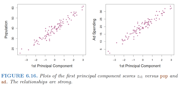
Figure 6.16 displays $z_{i1}$ versus both pop and ad. The plots show a strong relationship between the first principal component and the two features. In other words, the first principal component appears to capture most of the information contained in the pop and ad predictors.
Compute the first principal component
Assume that each of the variables in $X$ has been centered to have mean zero. We then look for the linear combination of the sample feature values of the form $$ \begin{align} z_{i1}=\phi_{11}x_{i1}+\phi_{21}x_{i2}+,,,+\phi_{p1}x_{ip} \quad \quad i=1,2,…,n \end{align} $$ that has largest sample variance, subject to the constraint that $\sum_{j=1}^p \phi_{j1}^2=1$
The first principal component loading vector solves the optimization problem $$ \begin{align} \max_{\phi_{11},…,\phi_{p1}} (\frac{1}{n} \sum_{i=1}^n \left( \sum_{j=1}^p \phi_{j1}x_{ij} \right)^2 ) , subject , to , \sum_{j=1}^p \phi_{j1}^2=1 \end{align} $$
Since $\sum_{i=1}^nx_{ij}/n=1$, the average of the $z_{11}, . . . , z_{n1}$ will be zero as well. Hence the objective that we are maximizing is just the sample variance of the $n$ values of zi1
Scores: We refer to $z_{11}, . . . , z_{n1}$ as the scores of the first principal component.
Geometric interpretation: for the first principal component: The loading vector $\phi_1$ with elements $\phi_{11},\phi_{21},…,\phi_{p1}$ defines a direction in feature space along which the data vary the most. If we project the n data points $x_1, . . . , x_n$ onto this direction, the projected values are the principal component scores $z_{11}, . . . , z_{n1}$ themselves.
2nd Principal Component
The second principal component $Z_2$ is a linear combination of the variables that is uncorrelated with $Z_1$, and has largest variance subject to this constraint.
It turns out that the zero correlation condition of $Z_1$ with $Z_2$ is equivalent to the condition that the direction must be perpendicular, or orthogonal, to the first principal component direction.
The second principal component is given by the formula:
$$ \begin{align} Z_2 = 0.544 × (pop − \bar{pop}) − 0.839 × (ad − \bar{ad}). \end{align} $$ Figure 6.15. The fact that the second principal component scores are much closer to zero indicates that this component captures far less information.
Compute the second principal component
The second principal component $Z_2$: the linear combination of $X_1,X_2, . . . , X_p$ that has maximal variance out of all linear combinations that are uncorrelated with $Z_1$.
The second principal component scores $z_{12}, . . . , z_{n2}$ take the form $$ \begin{align} z_{i2}=\phi_{12}x_{i1}+\phi_{22}x_{i2}+,,,+\phi_{p2}x_{ip} \quad \quad i=1,2,…,n \end{align} $$ where $\phi_2$ is the second principal component loading vector, with elements $\phi_{12},\phi_{22},…,\phi_{p2}$.
It turns out that constraining $Z_2$ to be uncorrelated with $Z_1$ is equivalent to constraining the direction $\phi_2$ to be orthogonal (perpendicular) to the direction $\phi_1$.
To find $\phi_2$, we solve a problem similar to (10.3) with $\phi_2$ replacing $\phi_1$, and with the additional constraint that $\phi_2$ is orthogonal to $\phi_1$
Interpretation:
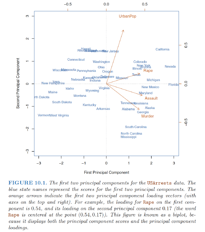
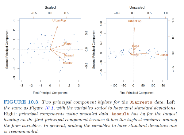
- 1st loading vector places approximately equal weight on Assault, Murder, and Rape, with much less weight UrbanPop. Hence this component roughly corresponds to a measure of overall rates of serious crimes.
- Overall, we see that the crime-related variables (Murder, Assault, and Rape) are located close to each other, and that the UrbanPop variable is far from the other three.
- This indicates that the crime-related variables are correlated with each other—states with high murder rates tend to have high assault and rape rates—and that the UrbanPop variable is less correlated with the other three.
Another Interpretation of Principal Components
An alternative interpretation for principal components: principal components provide low-dimensional linear surfaces that are closest to the observations
The first principal component loading vector has a very special property: it is the line in p-dimensional space that is closest to the n observations (using average squared Euclidean distance as a measure of closeness).
The appeal of this interpretation : we seek a single dimension of the data that lies as close as possible to all of the data points, since such a line will likely provide a good summary of the data.
The first two principal components of a data set span the plane that is closest to the n observations, in terms of average squared Euclidean distance
Together the first M principal component score vectors and the first M principal component loading vectors provide the best M-dimensional approximation (in terms of Euclidean distance) to the ith observation $x_{ij}$ . $$ \begin{align} x_{ij} \approx \sum_{m=1}^Mz_{im}\phi_{jm} \end{align} $$ (assuming the original data matrix X is column-centered).
When $M = min(n − 1, p)$, then the representation is exact: $x_{ij} = \sum_{m=1}^Mz_{im}\phi_{jm}$
More on PCA
Scaling the Variables
Before PCA is performed, the variables should be centered to have mean zero. Furthermore, the results obtained when we perform PCA will also depend on whether the variables have been individually scaled (each multiplied by a different constant)
Uniqueness of the Principal Components
**Each principal component loading vector $\phi_1=(\phi_{11},\phi_{21},…,\phi_{p1})^T$ and the score vectors $z_{11}, . . . , z_{n1}$ is unique, up to a sign flip. **
- Two different software packages will yield the same principal component loading vectors and score vectors, although the signs of those loading vectors may differ.
- The signs may differ because each principal component loading vector specifies a direction in p-dimensional space: flipping the sign has no effect as the direction does not change.
The Proportion of Variance Explained
How much of the variance in the data is not contained in the first few principal components?
Proportion of variance explained (PVE) by each principal component:
- The total variance present in a data set (assuming that the variables have been centered to have mean zero) is defined as
$$ \begin{align} \sum_{j=1}^pVar(X_j)=\sum_{j=1}^p\frac{1}{n}\sum_{i=1}^nx_{ij}^2 \end{align} $$
- The variance explained by the mth principal component is
$$ \begin{align} \frac{1}{n}\sum_{i=1}^nz_{im}^2=\frac{1}{n}\sum_{i=1}^n \left( \sum_{j=1}^p \phi_{jm}x_{ij} \right)^2 \end{align} $$
- Therefore, the PVE of the mth principal component is given by
$$ \begin{align} \frac{\sum_{i=1}^n \left( \sum_{j=1}^p \phi_{jm}x_{ij} \right)^2}{\sum_{j=1}^p\sum_{i=1}^nx_{ij}^2} \end{align} $$
The PVE of each principal component is a positive quantity. In order to compute the cumulative PVE of the first $M$ principal components, we can simply sum (10.8) over each of the first $M$ PVEs. In total, there are $min(n − 1, p)$ principal components, and their PVEs sum to one.

Deciding How Many Principal Components to Use
We would like to use the smallest number of principal components required to get a good understanding of the data.
How many principal components are needed?
- We typically decide on the number of principal components required to visualize the data by examining a scree plot (Right FIGURE 10.4)
- We choose the smallest number of principal components that are required in order to explain a sizable amount of the variation in the data.
- We tend to look at the first few principal components in order to find interesting patterns in the data. If no interesting patterns are found in the first few principal components, then further principal components are unlikely to be of interest.
The Principal Components Regression Approach
The principal components regression (PCR) approach involves constructing the first M principal components, $Z_1,Z_2, . . . ,Z_M$, and then using these components as the predictors in a linear regression model that is fit using least squares
The key idea
Often a small number of principal components suffice to explain most of the variability in the data, as well as the relationship with the response. In other words, we assume that the directions in which $X_1, . . .,X_p$ show the most variation are the directions that are associated with $Y$
Example:
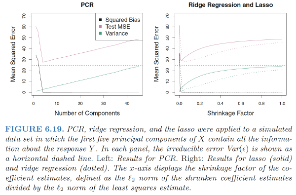
- Performing PCR with an appropriate choice of M can result in a substantial improvement over least squares
- PCR does not perform as well as the two shrinkage methods
- Reason: The data were generated in such a way that many principal components are required in order to adequately model the response. In contrast, PCR will tend to do well in cases when the first few principal components are sufficient to capture most of the variation in the predictors as well as the relationship with the response.
Note: even though PCR provides a simple way to perform regression using $M < p$ predictors, it is not a feature selection method!
- This is because each of the $M$ principal components used in the regression is a linear combination of all p of the original features.
- PCR is more closely related to ridge regression than to the lasso. One can even think of ridge regression as a continuous version of PCR!
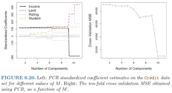
Cross-validation: In PCR, the number of principal components, $M$, is typically chosen by cross-validation.
Standardisation: When performing PCR, we generally recommend standardizing each predictor, prior to generating the principal components.
- In the absence of standardization, the high-variance variables will tend to play a larger role in the principal components obtained, and the scale on which the variables are measured will ultimately have an effect on the final PCR model.
Ref:
James, Gareth, et al. An introduction to statistical learning. Vol. 112. New York: springer, 2013.
Hastie, Trevor, et al. “The elements of statistical learning: data mining, inference and prediction.” The Mathematical Intelligencer 27.2 (2005): 83-85