Logistic regression and LDA methods are closely connected.
Setting: Consider the two-class setting with \(p = 1\) predictor, and let \(p_1(x)\) and \(p_2(x) = 1−p_1(x)\) be the probabilities that the observation \(X = x\) belongs to class 1 and class 2, respectively.
In LDA, from
$$ \begin{align} p_k(x)=\frac{\pi_k \frac{1}{\sqrt{2\pi}\sigma}\exp{\left( -\frac{1}{2\sigma^2}(x-\mu_k)^2 \right)}}{\sum_{l=1}^K\pi_l\frac{1}{\sqrt{2\pi}\sigma}\exp{\left( -\frac{1}{2\sigma^2}(x-\mu_l)^2 \right)}} \end{align} $$
$$ \begin{align} \delta_k(x)=x\frac{\mu_k}{\sigma^2}-\frac{\mu_k^2}{2\sigma^2}+\log(\pi_k) \end{align} $$ The log odds is given by
$$ \begin{align}\log{\frac{p_1(x)}{1-p_1(x)}}=\log{\frac{p_1(x)}{p_2(x)}}=c_0+c_1x \end{align} $$ where c0 and c1 are functions of μ1, μ2, and σ2.
In Logistic Regression,
$$ \begin{align} \log{\frac{p_1}{1-p_1}}=\beta_0+\beta_1x \end{align} $$
SAME
- Both logistic regression and LDA produce linear decision boundaries.
DIFFERENCES
The only difference between the two approaches lies in the fact that β0 and β1 are estimated using maximum likelihood, whereas c0 and c1 are computed using the estimated mean and variance from a normal distribution. This same connection between LDA and logistic regression also holds for multidimensional data with p > 1.
LDA assumes that the observations are drawn from a Gaussian distribution with a common covariance matrix in each class, and so can provide some improvements over logistic regression when this assumption approximately holds. Conversely, logistic regression can outperform LDA if these Gaussian assumptions are not met.
KNN dominate LDA and Logistic in non-linear setting
In order to make a prediction for an observation X = x, the K training observations that are closest to x are identified. Then X is assigned to the class to which the plurality of these observations belong. Hence KNN is a completely non-parametric approach: no assumptions are made about the shape of the decision boundary.
Therefore, we can expect KNN to dominate LDA and logistic regression when the decision boundary is highly non-linear.
On the other hand, KNN does not tell us which predictors are important
QDA serves as a compromise between KNN, LDA and logistic regression
QDA serves as a compromise between the non-parametric KNN method and the linear LDA and logistic regression approaches. Since QDA assumes a quadratic decision boundary, it can accurately model a wider range of problems than can the linear methods. Though not as flexible as KNN, QDA can perform better in the presence of a limited number of training observations because it does make some assumptions about the form of the decision boundary.
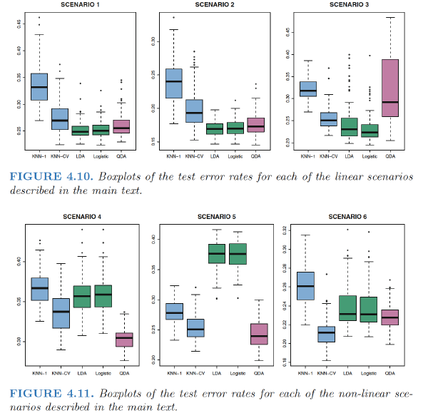
Scenario 1: - 20 training observations in each of two classes. The observations within each class were uncorrelated random normal variables with a different mean in each class. - LDA performed well in this setting. KNN performed poorly because it paid a price in terms of variance that was not offset by a reduction in bias.
Scenario 2: - Details are as in Scenario 1, except that within each class, the two predictors had a correlation of −0.5. - Little change in the relative performances of the methods as compared to the previous scenario.
Scenario 3: - X1 and X2 are from the t-distribution, with 50 observations per class.
The t-distribution has a similar shape to the normal distribution, but it has a tendency to yield more extreme points—that is, more points that are far from the mean.
- The decision boundary was still linear, and so fit into the logistic regression framework. The set-up violated the assumptions of LDA, since the observations were not drawn from a normal distribution. QDA results deteriorated considerably as a consequence of non-normality.
Scenario 4: - The data were generated from a normal distribution, with a correlation of 0.5 between the predictors in the first class, and correlation of −0.5 between the predictors in the second class. - This setup corresponded to the QDA assumption, and resulted in quadratic decision boundaries.
Scenario 5: - Within each class, the observations were generated from a normal distribution with uncorrelated predictors. However, the responses were sampled from the logistic function using \(X^2_1 , X^2_2, and \, X1 × X2\) as predictors. - Consequently, there is a quadratic decision boundary. QDA once again performed best, followed closely by KNN-CV. The linear methods had poor performance.
Scenario 6: - Details are as in the previous scenario, but the responses were sampled from a more complicated non-linear function. - Even the quadratic decision boundaries of QDA could not adequately model the data. - Much more flexible KNN-CV method gave the best results. But KNN with K = 1 gave the worst results out of all methods.
This highlights the fact that even when the data exhibits a complex nonlinear relationship, a non-parametric method such as KNN can still give poor results if the level of smoothness is not chosen correctly.
Conclusion
When the true decision boundaries are linear, then the LDA and logistic regression approaches will tend to perform well.
When the boundaries are moderately non-linear, QDA may give better results.
For much more complicated decision boundaries, a non-parametric approach such as KNN can be superior. But the level of smoothness for a non-parametric approach must be chosen carefully.
Ref:
James, Gareth, et al. An introduction to statistical learning. Vol. 112. New York: springer, 2013.
Hastie, Trevor, et al. “The elements of statistical learning: data mining, inference and prediction.” The Mathematical Intelligencer 27.2 (2005): 83-85