Bias, Variance and Model Complexity
Test error (generalization error): the prediction error over an independent test sample
$$ \begin{align} Err(\tau)=E[L(Y,\hat{f} (X))|\tau] \end{align} $$
Here the training set $\tau$ is fixed, and test error refers to the error for this specific training set.
Expected test error: $$ Err=E[L(Y,\hat{f}(X)]=E[Err_\tau] $$
This expectation averages over everything that is random, including the randomness in the training set that produced $\hat{f}$
Training error: the average loss over the training sample $$ \bar{err}=\frac{1}{N}\sum_{i=1}^NL(y_i,\hat{f}(x_i)) $$

Model selection: estimating the performance of different models in order to choose the best one.
Model assessment: having chosen a final model, estimating its prediction error (generalization error) on new data.
Randomly divide the dataset into three parts:
- a training set: fit the models
- a validation set: estimate prediction error for model selection
- a test set: assessment of the generalization error of the nal chosen model
A typical split might be 50% for training, and 25% each for validation and testing:
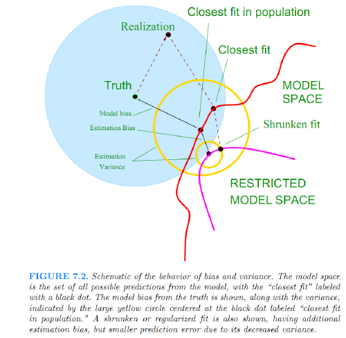
The Bias Variance Decomposition
General Model
If we assume that $Y=f(X)+\epsilon$ where $E(\epsilon)=0$, and $Var(\epsilon)=\sigma^2_\epsilon$, we can derive an expression for the expected prediction error of a regression fit $\hat{f}(X)$ at an input point X = x0, using squared-error loss:
$$ \begin{align} Err(x_0)&=E[(Y-\hat{f}(x_0))^2|X=x_0] \\ &=E[(f(x_0)+\epsilon-\hat{f}(x_0))^2] \\ &=E[\epsilon^2+(f(x_0)-\hat{f}(x_0))^2+2\epsilon(f(x_0)-\hat{f}(x_0))] \\ &=\sigma^2_\epsilon+E[f(x_0)^2+\hat{f}(x_0)^2-2f(x_0)\hat{f}(x_0)] \\ &=\sigma^2_\epsilon+E[\hat{f}(x_0)^2]+f(x_0)^2-2f(x_0)E[\hat{f}(x_0)] \\ &=\sigma^2_\epsilon+(E[\hat{f}(x_0)])^2+f(x_0)^2-2f(x_0)E[\hat{f}(x_0)] +E[\hat{f}(x_0)^2]-(E[\hat{f}(x_0))^2 \\ &=\sigma^2_\epsilon+(E\hat{f}(x_0)-f(x_0))^2+Var(\hat{f}(x_0))\\ &=\sigma^2_\epsilon+Bias^2(\hat{f}(x_0))+Var(\hat{f}(x_0))\\ &= Irreducible Error+ Bias^2 + Variance \end{align} $$
- The first term is the variance of the target around its true mean f(x0), and cannot be avoided no matter how well we estimate f(x0), unless $\sigma^2_\epsilon=0$
- The second term is the squared bias, the amount by which the average of our estimate differs from the true mean
- The last term is the variance; the expected squared deviation of $\hat{f}(x_0)$ around its mean.
Typically the more complex we make the model $\hat{f}$, the lower the (squared) bias but the higher the variance.
KNN regression
For the k-nearest-neighbor regression t, these expressions have the sim-
ple form
$$
\begin{align}
Err(x_0)&=E[(Y-\hat{f}_k(x_0))^2|X=x_0] \
\end{align}
$$
Ref:
James, Gareth, et al. An introduction to statistical learning. Vol. 112. New York: springer, 2013.
Hastie, Trevor, et al. “The elements of statistical learning: data mining, inference and prediction.” The Mathematical Intelligencer 27.2 (2005): 83-85